Charts
42 chart kinds. A chart is the cast on the measure column; the other columns of the SELECT say where and how each row is drawn. Pick by the question: compare amounts → bars; change over time → lines; a relationship → points; spread → distributions; shares and flows → part of a whole; geography → maps.
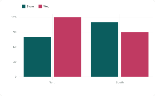
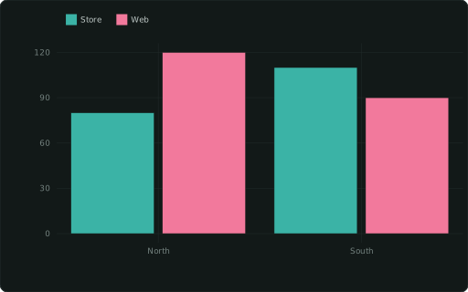
::BARCHARTbar chart (dodged by CATEGORY)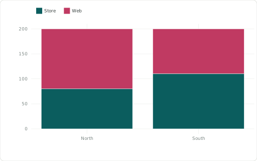
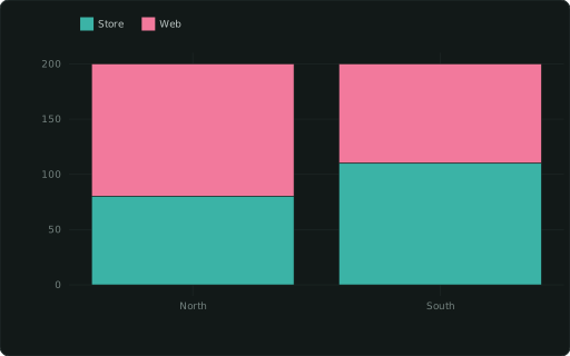
::BARCHART_STACKEDstacked bars (by CATEGORY)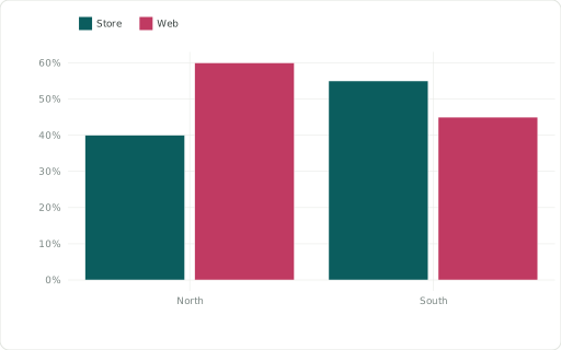
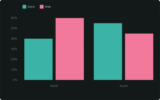
::BARCHART_PERCENTdodged bars as % of each x’s total (fractions ≤ 1 are drawn as given)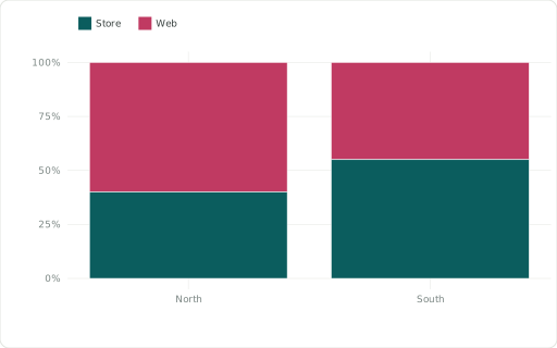
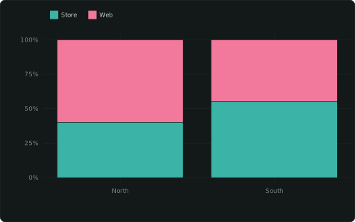
::BARCHART_STACKED_PERCENTbars normalised to 100% per x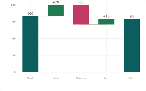
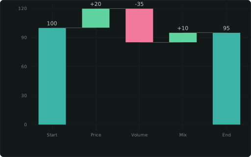
::WATERFALLbridge from a start total through signed steps (NULL / ::CATEGORY ‘total’ rows = totals)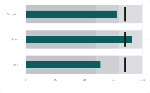
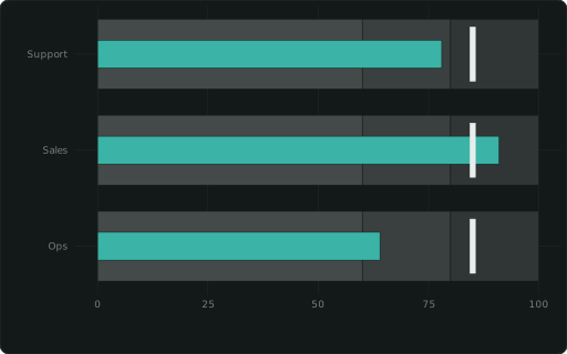
::BULLETmeasure per XAXIS row vs a ::GOAL tick over ::RANGE bands ‘60,80,100’

::FUNNELordered XAXIS stages, widths by value, conversion % from the previous stage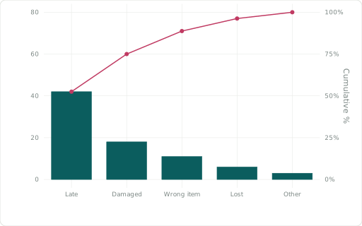
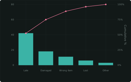
::PARETOXAXIS categories as bars sorted largest first, with the cumulative share as a line on a 0–100 % right axis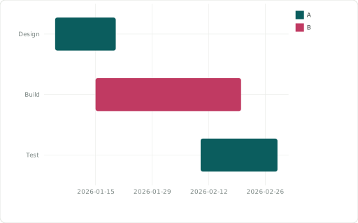
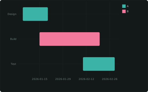
::GANTTone bar per task (this column names it) from ::XMIN to ::XMAX (dates or numbers); ::CATEGORY colours the bars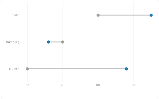
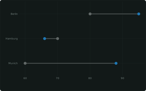
::DUMBBELLtwo values per item (this column names it) joined by a line: ::XMIN → ::XMAX (before/after, plan/actual)Lines and areas
Section titled “Lines and areas”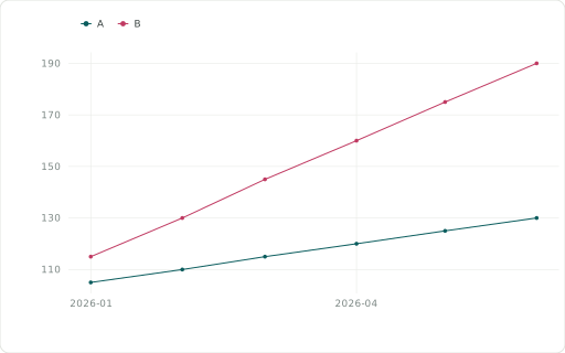
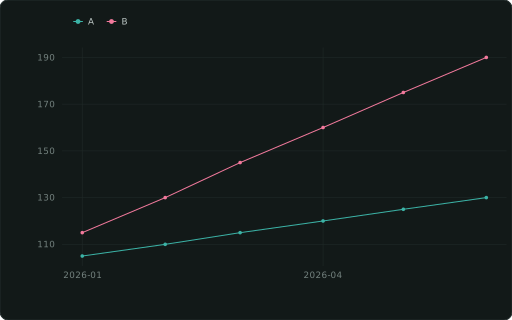
::LINECHARTline chart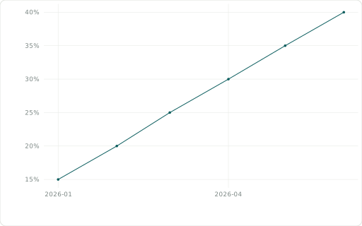
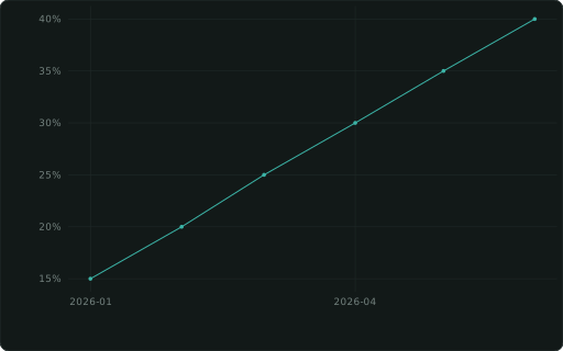
::LINECHART_PERCENTline chart, percent y-axis

::STEPstep line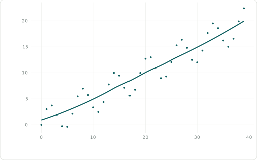
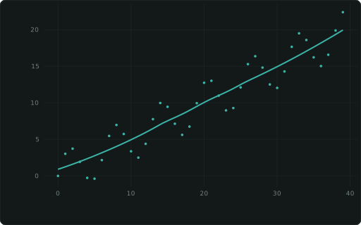
::SMOOTHscatter + trend line (LOESS; ::SMOOTH_METHOD ‘lm’/‘gam’)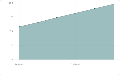
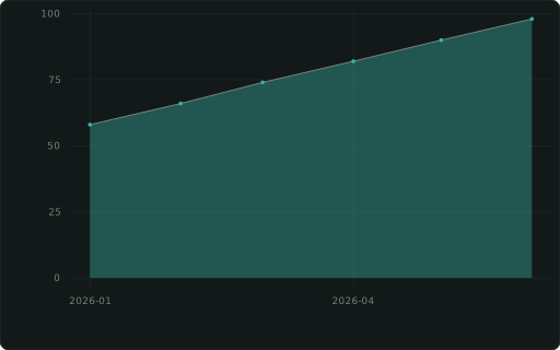
::AREACHARTarea chart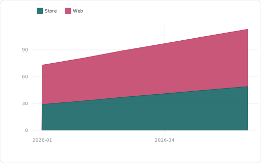
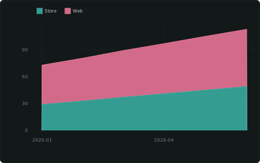
::AREACHART_STACKEDstacked areas (by CATEGORY)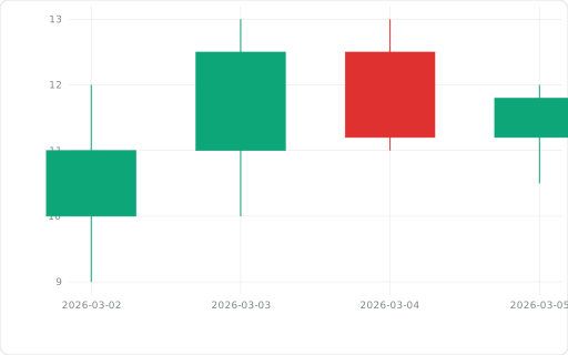
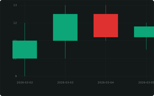
::CANDLESTICKOHLC candlesticks: XAXIS + ::OPEN/::HIGH/::LOW, close as the measure

::SPARKLINEminimal trend line (no axes); a list() column in a table; on a map: a mini chart in each feature’s tooltip

::SPARKBARminimal bar histogram (no axes); a table cell’s list(v ORDER BY i), or two overlaid series sharing one y scale from list(‘ref’: r, ‘cur’: c ORDER BY i); on a map: a mini chart in each feature’s tooltipPoints
Section titled “Points”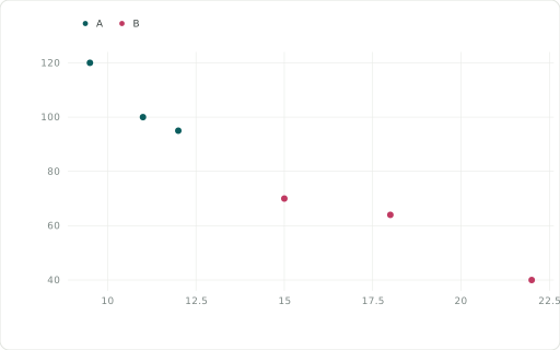
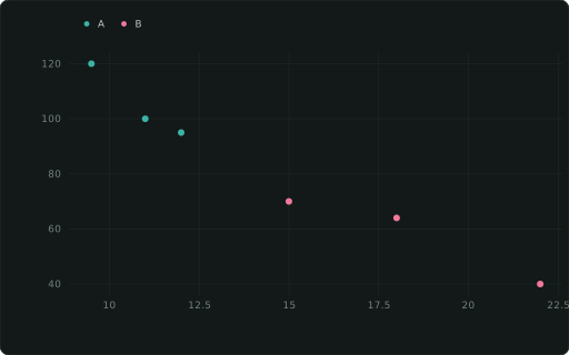
::SCATTERscatter; add a ::SIZE column for a bubble chart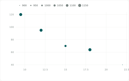
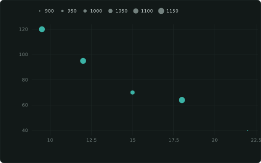
::BUBBLEbubble chart: alone = the y measure (size via ::SIZE); beside a ::SCATTER = its size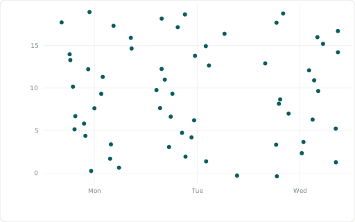
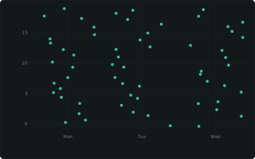
::JITTERjittered scatter (reveals overlapping points)Distributions
Section titled “Distributions”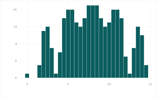
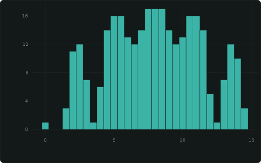
::HISTOGRAMhistogram of the measure; takes ::FLIP (horizontal, with ::FACET panels too), ::YFORMAT / ::YSCALE on its count axis, ::DATALABELS (each bin’s count, or share under ::HIST_NORM), ::ABLINE, ::XLINE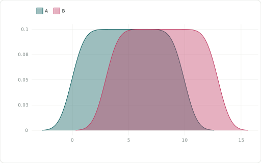
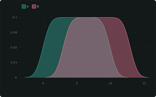
::DENSITYkernel density curve (one per CATEGORY)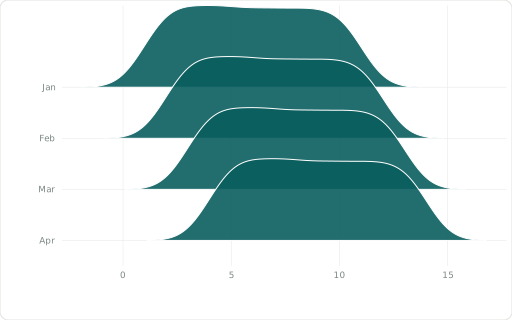
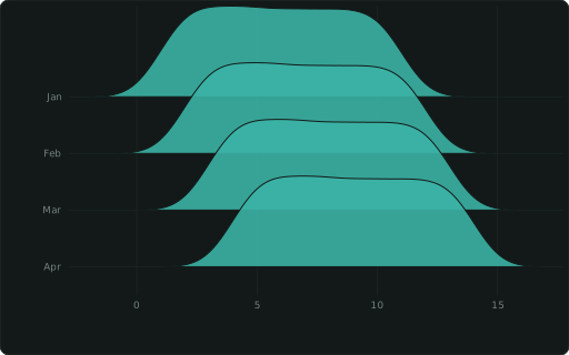
::RIDGELINEone density of the measure per ::CATEGORY, stacked as overlapping ridges (distributions over time; the first category on top)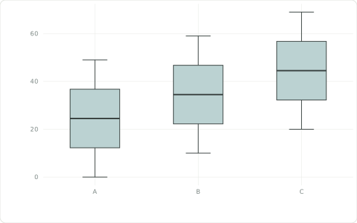
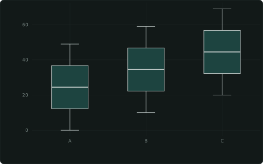
::BOXPLOTbox plot — XAXIS groups, measure on y (raw rows)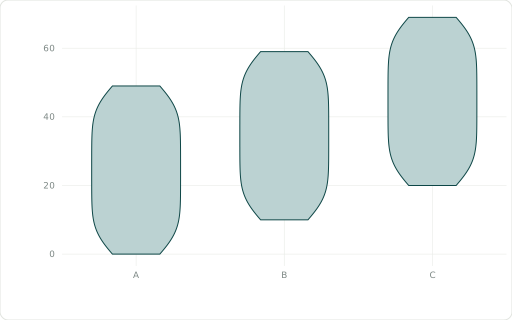
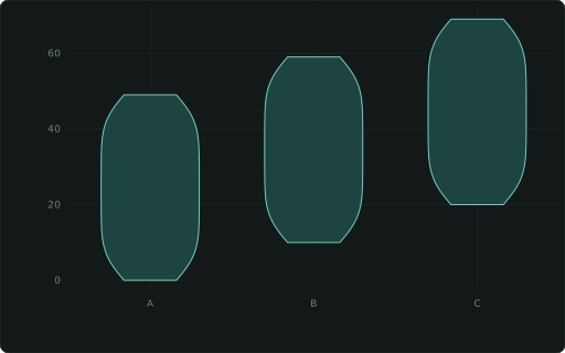
::VIOLINviolin plot — XAXIS groups, measure on y (raw rows)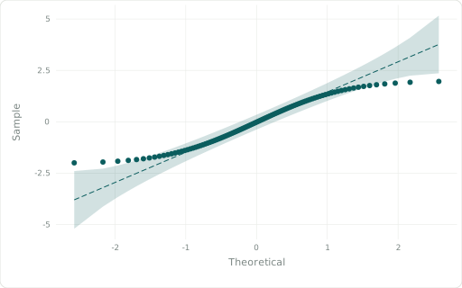
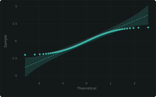
::QQnormal quantile-quantile plot with a 95% pointwise bandPart of a whole and flows
Section titled “Part of a whole and flows”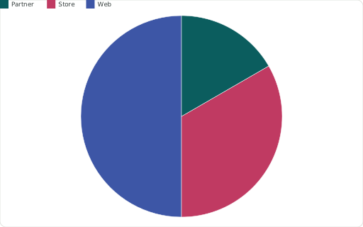
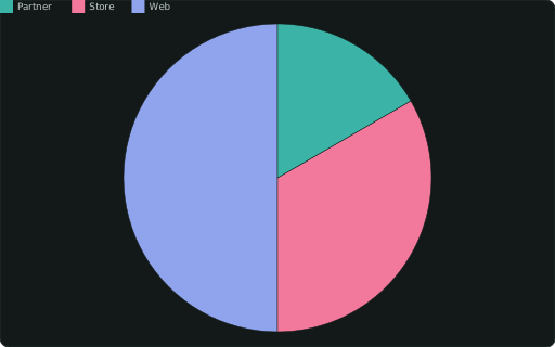
::PIEpie — slices by CATEGORY, sized by the measure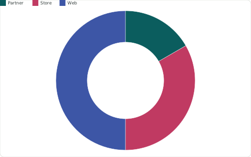
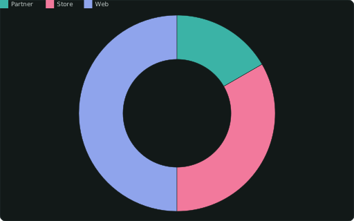
::DONUTCHARTdonut (pie with a hole)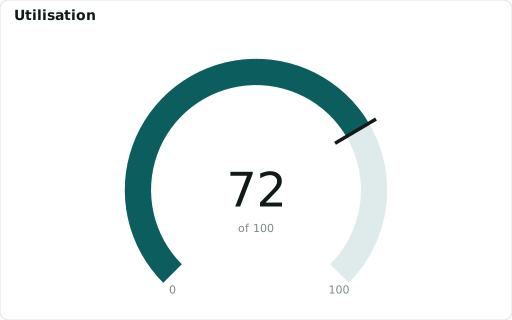
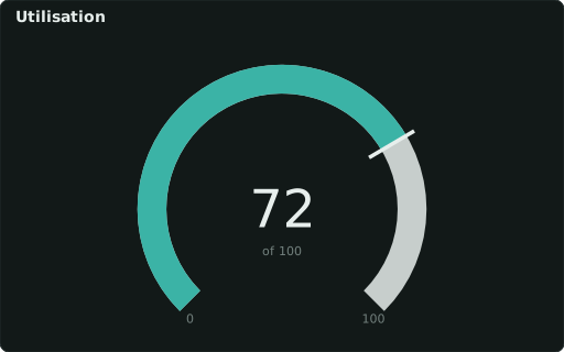
::GAUGEvalue as an arc toward ::RANGE ‘min,max’ (zones: ::COLORS, ::LABELS)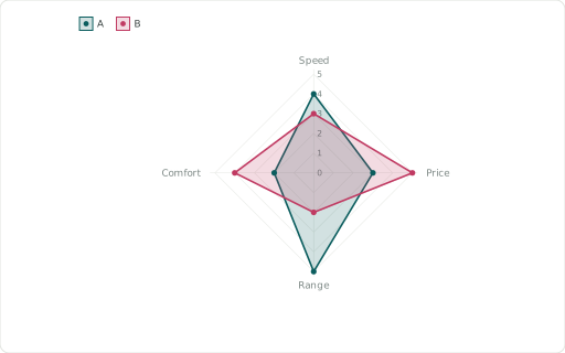
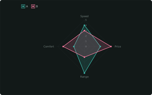
::RADARradar / spider chart — axes from XAXIS, one polygon per CATEGORY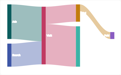
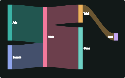
::SANKEYflows between stages: ::ORIGIN → ::DEST, link width by the measure; nodes stack in columns

::TREEMAPpart-to-whole tiles, area by the measure: ::XAXIS names a tile (its key; a ::LABEL then shows a name instead), ::CATEGORY nests tiles in groups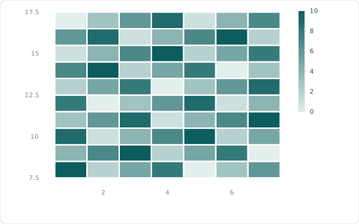
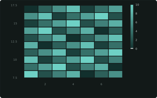
::HEATMAPtiles at XAXIS×YAXIS coloured by the measure (rows in SQL order; diverging around 0); a numeric measure sizes every tile alike regardless of how many x points each row has; a text measure (status words) takes ::COLORS as a level map for a categorical legend, like a ::CATEGORY column’s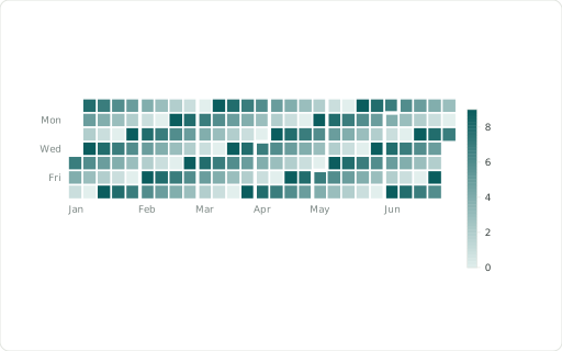
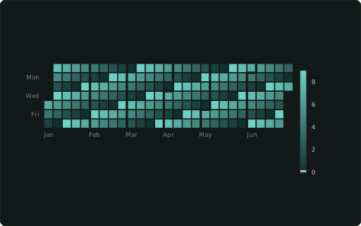
::CALENDARcalendar heatmap (date XAXIS, ≤ 50 years)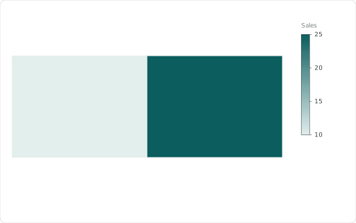
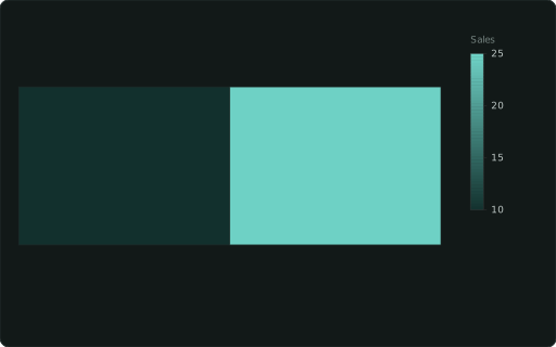
::MAPWKT-geometry map, coloured by a measure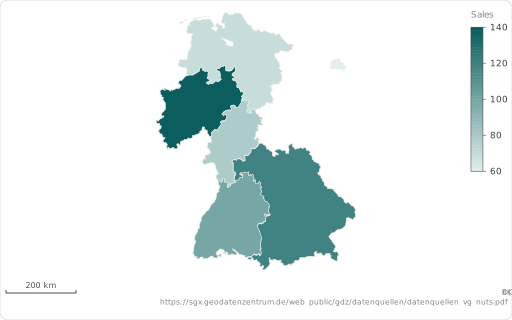
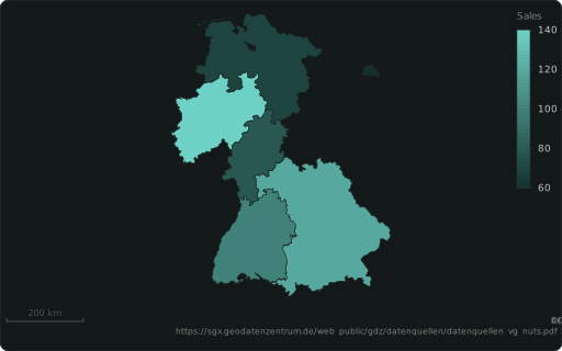
::REGIONa map region by code, drawn from the built-in boundaries: ISO 3166-1 (‘DE’, ‘DEU’), ISO 3166-2 (‘DE-BY’, ‘US-CA’: states and provinces everywhere), German AGS (‘09162’) or NUTS (‘DE212’), else a name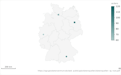
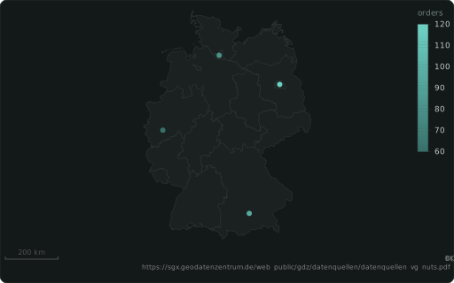
::LAT + ::LONa map point’s latitude (degrees, WGS84), with ::LON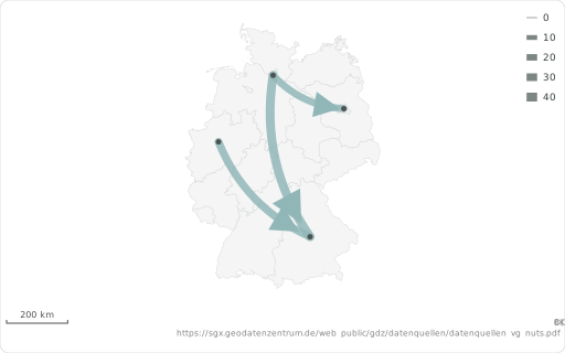
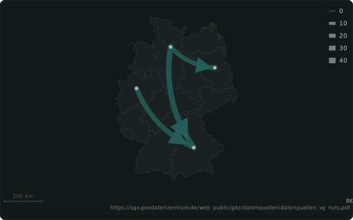
::ORIGIN + ::DESTa flow map’s start: a region code (‘DE-BY’), a WKT POINT or ‘lon’: …, ‘lat’: …, ‘name’: … — with ::DEST, width by ::SIZE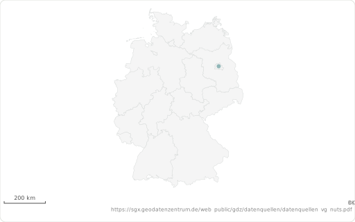
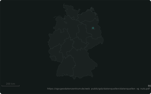
::BASEMAPa backdrop under a map: WKT, or a built-in layer ‘world’, ‘de-states’, ‘de-districts’